by
Peter Dietze
![]()
`Open Review' comments were invited on this paper and on the subject of carbon modelling generally.
That discussion remains available at the following link.
by
Peter Dietze
![]()
`Open Review' comments were invited on this paper and on the subject of carbon modelling generally.
That discussion remains available at the following link.
IPCC's emissions scenario IS92a is used as first input to a simple carbon model, parametrized in four different ways. A second simulation is performed with IS92aD, a reality-adapted IS92a scenario which peaks at 12 GtC/yr around 2040 and then reduces emissions until all the usable 1,300 GtC are burnt in 2150. The CO2 concentration perfectly matches present observations and does not increase to more than 470 ppm. The airborne fraction reduces to near zero in 2070. The third simulation uses the SRES A1 scenario from IPCC TAR. Eyestriking exaggerations of IPCC's Bern model results (677 vs. 540 ppm) and an unrealistic CO2 lifetime of 570 years are revealed being confirmed as well by a WRE550 stabilization scenario run showing a seven times too high CO2 increment. Essential discussions are presented.
The author's carbon model has been developed since 1992. Publications were in 1995 in German [Energiew. Tagesfr. 45, 329, 5], 1997 in English at John Daly's site, 1998 in German [Klima 2000 2, 24-35, 5/6] and at Peter Krahmer's site and 2000 in Chapter 2 of the author's official TAR Review. The model computes the CO2 concentration incrementally, only using the past emissions and a scenario for the future, starting from a flat state concentration (for example 280 ppm in 1840). The model approach uses a best-match CO2 excess lifetime of 55 yr and besides the atmosphere an auxiliary buffer that is best-fit estimated to be 33% of the atmosphere's capacity. So not 2.123 GtC, but 33% more have to be injected as an emission impulse to increase the CO2 concentration by 1 ppm before the natural sequestration works. The half-life time of any partial pressure increment is 55·ln(2)=38 years. The global CO2 uptake (sum of oceans and biomass sink flows) is principally assumed to be roughly proportional to the increment in partial pressure against the equilibrium concentration. The system is thus being linearized within the observed operating regime.
The model's math procedure solves a simple first order differential equation by convolution integral in a sequential mode. This means application of an e-functional decay to the existing total CO2 mass in the global buffer (atmosphere, surface water etc.) and a CO2 increment from emissions for each time interval. The model has been easily implemented in Excel. For this paper 5yr intervals have been chosen (a finer resolution is not required for a long term simulation), all data points being located at the middle of each interval. For example the 1995 interval covers 1993..1997. So if individual emissions for each of these five years are given, they are summed up to make one emission impulse for the 1995 interval. The CO2 concentration is calculated for yr 1995, 2000 and so on.
In February 2001 tests were run to approximate and compare the model results with IPCC's response for scenario IS92a and subsequently with their responses for SRES A1 and WRE550 which are used in the Third Assessment Report (TAR). The test results were mailed to some well known carbon modellers, among them Prof. Jan Goudriaan, Prof. Tom Wigley, Dr. Brian O'Neill and Dr. Fortunat Joos (he prepared the Bern carbon model runs for the IPCC TAR). The correspondence and further comments are within this paper.
~~~~~
Peter Dietze wrote to Prof. Jan Goudriaan: (13 February 2001, CC to Dr. Fortunat Joos)
Dear Prof. Goudriaan,
recently I have done some carbon model calculations that may be interesting for you. I use Excel to implement my system differential equation and to perform the convolution integral to calculate the CO2 concentration (see my model documentation in chapter 2 at http://www.john-daly.com/forcing/moderr.htm).
In Fig.1 you find the past total emissions, with CDIAC data after 1970 till 1995 and IS92a till 2100. The CO2 concentrations are computed 4-fold with
a) Dietze's model (buffer fraction BF=75%,
e-fold
lifetime T=55yr),
b) IPCC approximation (BF=48%, T=infinite), ending at 708 ppm in 2100
c) IPCC approximation (BF=53%, T=570yr), ending at 704 ppm in 2100
d) Goudriaan's model (BF=64%, T=120yr)
The IPCC approximation c) has been worked out because the Bern model yields small sink flows at the end, about 2 GtC/a. Here a best-fit effective lifetime of 570 yr is applied [see Fig.5 which is in great contrast to the 120yr often cited by IPCC]. Approximation c) was necessary because b) would yield no sink flows but only accumulation which is not realistic to approximate the IPCC (Bern) carbon model.
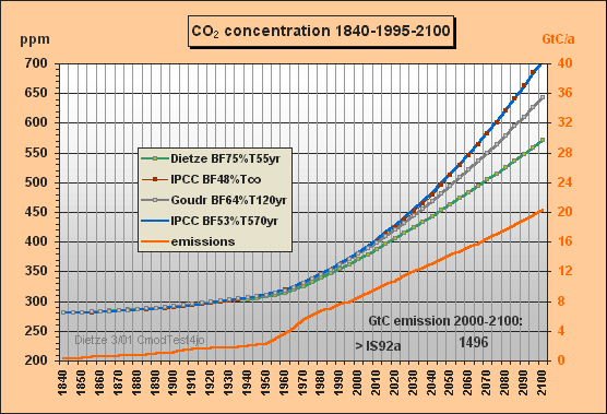
Fig.1: Model results for the a) Dietze, b) and c) IPCC
and d) Goudriaan model
approximations for IS92a total emissions scenario
till 2100
Fig.2 shows the second carbon model test. The parameters from c), i.e. BF=53% and T=570yr, are used to solve for my total emissions scenario IS92aD, i.e. IS92a until 2030, but then reducing emissions (e.g. thorium breeders are taking over), but in total burning the usable fossil reserves of some 1300 GtC until 2150.
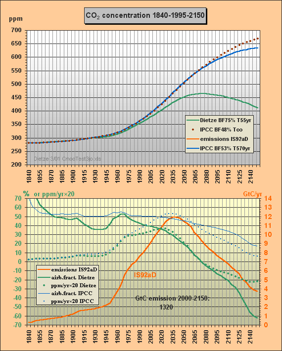
Fig.2: Model results for the a) Dietze, b) and c) IPCC
model
approximations for IS92aD emissions scenario till
2150
Here the CO2 concentrations are computed with my model a) and for the two different IPCC approximations b) and c). Eyestriking differences can be seen between my results (green) and the IPCC Bern approximation with small sink flows (blue). The IPCC approximation with infinite lifetime, i.e. with a constant 48% airborne fraction, is indicated as well (brown, dotted).
Best regards,
Peter Dietze
~~~~~
Comments:
Whereas the IPCC Bern model approximation c) peaks at a concentration of 634 ppm (blue), my model peaks at 465 ppm only, which is 95 ppm less than a CO2 doubling, though all usable fossil fuel being estimated as about 1300 GtC is burnt until 2150. At the time of correspondence with Prof. Goudriaan and Dr. Joos Fig.2 only showed the IS92aD emissions for this second test. Meanwhile the 260 yr lifetime, previously used to simulate the Bern model, has been corrected to best fitting 570 years. Moreover Fig.2 has been extended for the airborne fractions and the yearly CO2 ppm increment to provide more insight to the different model characteristics and thus to support validation. Note that the airborne fraction is defined in this paper as the ratio betweeen the yearly growth of the atmospheric carbon content omitting the auxiliary buffer and the total emissions (fossil plus land use).
Around yr 2000 my model reproduces the observed 369 ppm though the computation is based on a long sequential mix of integration and decay, starting in 1840. Note that the procedure uses nothing but the total emissions data for the middle of each 5yr interval, i.e. not any other observations are used for internal 'upgrading' of intermediate results. Between 1975 and 2000 my model yields a rather stable yearly CO2 increment of 1.5 ppm (as observed), wheras IPCC's rises to 2.1 ppm.
The airborne fraction behaviour is most interesting. IPCC's fraction stays around 50% between 1915 and 2020. In my model the fraction is drastically reducing since 1965 though the emissions were increasing considerably. IPCC's fraction curbs only little so that with increasing emissions the CO2 increment is rising to 2.7 ppm/yr in 2030 (dotted blue curve) whereas my increment is 1.7 ppm only. Remarkable is that around 2070 my airborne fraction reduces to zero (ie. all 9.4 GtC emissions will be sequestered) and further on even turns to negative (i.e. sequestration outweighs emissions). For the IPCC Bern model this break-even point is not even reached in 2150 because of the small sink flux.
For the third carbon model test and to obtain a direct response intercomparison with IPCC, the SRES A1 emissions scenario was chosen in spite of the emissions increment for the next two decades being unrealistically high. Fig.3 shows the SRES scenarios that Dr. Joos used for the diagrams in the IPCC TAR. The Bern model results which have been submitted for the TAR, are shown in Fig.4.
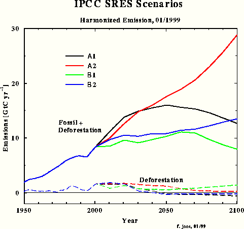
Fig.3: SRES scenarios used by Dr. Joos for the IPCC TAR
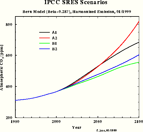
Fig.4: Bern model results for SRES scenarios
With the SRES A1 emissions data as input the CO2 concentrations were calculated till 2100, using the IPCC model approximation c) based on the best-fit set of buffer fraction BF=53% and lifetime T=570yr in comparison to my model (Fig.5).
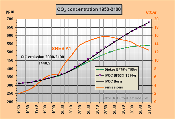
Fig.5: Model results for the a) Dietze and c) IPCC
Bern model
approximation for SRES A1 emissions scenario till
2100
This simulation shows that my outmost simple IPCC Bern model approximation for SRES A1 yields a response function (purple) which is almost identical with the one in Fig.4 calculated by the original Bern model (black). The max concentration in 2100 is 679 ppm. In comparison with my model's result peaking at 540 ppm only, IPCC's concentration increment (related to 1950) is exaggerated by 60 %. If we take an equilibrium climate sensitivity of 0.7 °C for CO2 doubling and a concentration increment from 310 to 540 ppm, the equilibrium warming for 1950-2100 will be only 0.55 °C.
Fig.5 reveals that the IPCC Bern model is indeed operating with an extremely high CO2 excess lifetime of 570yr so that this model has very small sink flows1) and mostly acts as emissions integrator. As only about 53% of the emissions instantaneously appear in the atmosphere, the Bern model has to use an auxiliary buffer which picks up the other 47%. This means, we would have to release 2.123/0.53 = 4.0 GtC for a 1 ppm instantaneous increment. The carbon that does not appear in the atmosphere, is usually and erroneously understood by IPCC people as being fastly absorbed. The 47% auxiliary buffer (equivalent to 89% of the atmosphere) is the reason why in spite of too small sink flows the Bern model is able to reproduce past observed concentrations (see the IS92a approximation in Fig.1). But too small sink flows are the cause for unrealistical high concentrations in the future.
The misinterpretation of this 47% buffer
flux as a sink flux seems to be the reason
why IPCC people permanently have problems to define a proper CO2
excess lifetime and keep emphasizing that any (effective or apparent) lifetime
must
be a ficticious mean value between different time scales of fast,
medium and slow sequestration. The function of the auxiliary buffer and
the question where it may be located, was never discussed in public. Obviously
it is mostly the mixed upper layer of the oceans
(apart from some biomass and soil contribution) which works as to enlarge
the buffer capacity of the atmosphere. Further we find the IPCC conviction,
CO2 will only slowly migrate deeper from the mixed
layer, i.e. mostly through
eddy
diffusion processes2).
This feature is indeed the key for understanding
IPCC's SAR statement (cited by Dr. O'Neill, see below) about a strange
sudden lifetime jump in case we would reduce the emissions: "However,
if emissions were reduced, the CO2 in the vegetation
and ocean surface water would soon equilibrate with that in the atmosphere,
and the rate of removal would then be determined by the slower response
of woody vegetations, soils, and transfer into the deeper layers of the
ocean". Actually, this is imagination as the rate of removal does not
at all depend on emissions (which nature is unable to detect), but only
depends on the partial pressure increment.
---
1) For example
assume stabilization at a concentration increment
from 280 ppm equilibrium to a 560 ppm level. As the buffer flux is zero,
the sink flow can be calculated from the total buffer excess i.e. atmospheric
excess devided by 0.53 which has to be devided by 570yr lifetime. 280·2.123/0.53/570
yields a sink flow of 2 GtC/yr which indeed
matches IPCC's stabilization scenarios. In contrast my model would if
a doubling could be reached at all stabilize at about 14
GtC/yr, i.e. seven times more.
2) To transport CO2 in the IPCC eddy diffusion model, a concentration gradient and a permanently increasing atmospheric concentration is required thus yielding a strong tendency of slowing down the uptake. In reality the main sink function performs quite different. Within the cold deep water formation CO2 is just dissolved and taken down without a gradient being necessary.
~~~~~
Response by Dr. Fortunat Joos: (20 February 2001)
P. Dietze wrote:
> Dear Prof. Goudriaan,
> recently I have done some carbon model calculations that may be
> interesting for you
> the IPCC approximation with small sink flows (blue) and with assumed
> constant airborne fraction and accumulation only (brown).
Dear Mr. Dietze,
You may plot for each of the IS92a-f series and the SRES serie 'CO2' vs 'emissions' and you will find that airborne fraction is not assumed constant as pointed out in earlier e-mails. The data are on my home page given below.
It would be nice if at some point in time you take the effort to read and trying to understand state-of-the-art publications on carbon cycle modelling and state-of-the-art publications on tracer observations (WOCE, GEOSECS, ..) within the ocean and on carbonate chemistry (DOE Handbook, Dickson, Roy et al. ...).
Regards,
Fortunat Joos
Fortunat Joos, Climate and Environmental Physics
Sidlerstr. 5, CH-3012 Bern
Phone: ++41(0)31 631 44 61 new Fax: ++41(0)31
631 87 42
e-mail: joos@climate.unibe.ch
Internet: http://www.climate.unibe.ch/~joos/
(relevant papers are listed here)
~~~~~
Response by Prof. Jan Goudriaan: (21 February 2001)
This is a response to an E-mail message of Peter Dietze and to a subsequent message of Dr. Joos. In the graph with model calculations that Peter Dietze distributed by E-mail, he presented a line which he ascribed to me. Indeed, I have once given him a set of just two equations that do a reasonable job in describing the response of the atmospheric CO2 concentration to an assumed emission. At that time I was in discussion with him, trying to understand what he is doing, and showing him my own simplified equations. I did this, because we had developed similar simplifying equations and felt that we had similar thinking so far. However, Mr. Dietze failed to see the limited validity of these simplifications. For instance, they do not allow for the increase of the buffer factor of ocean water after it has absorbed a lot of CO2. Because of this, these equations tend to slightly underestimate the prognosis of atmospheric CO2 concentration beyond 600 ppm or so.
I should emphasize that my own complete model produces results that are very close to the IPCC prognosis.
I have run Dietze's model parallel to my own code, reproducing almost exactly what he has sent around. However, in my opinion Dietze's model is absolutely beside the truth. Mr. Dietze treats CO2 as if it disappears from the atmosphere with a time coefficient of 55 years. This assumes that somehow the earth system can destroy or sequester CO2 completely at such a fast rate.
The problem is that is very hard to discriminate the models on the basis of present atmospheric CO2 observation alone, because so far the dynamic responses of both model formulations are very close. They begin to diverge only later. However, they do differ a lot in other respects which can be checked right now. One of these is the oceanography, as Dr Joos rightly points out, and another one is for instance isotope behaviour. I do hope that Mr. Dietze will be willing to look at these fields.
Jan Goudriaan
One of his relevant papers:
Goudriaan, J.: 1993, 'Interaction of ocean and biosphere in their transient responses to increasing atmospheric CO2', Vegetatio 104/105, 329-337.
~~~~~~~
Peter Dietze's answer to Dr. Fortunat Joos: (22 February 2001)
Dear Dr. Joos,
thanks for your response on 20 February. You wrote
> You may plot for each of the IS92a-f series and the SRES serie
> 'CO2' vs 'emissions'
and you will find that airborne fraction is not
> assumed constant as pointed out in earlier
e-mails
There is a misinterpretation of yours. Formerly Dr. Ahlbeck found that IPCC's carbon model response on IS92a looks nearly as if just assuming a constant airborne fraction of about 50%. In my email "Carbon Model calculations" on 13 February I showed that a rather good match is 48% (with lifetime T being infinite). As I know that your model indeed does not use such a simple approximation, I wrote:
> a) Dietze's model (buffer fraction BF=75%,
e-fold lifetime T=55yr)
> b) IPCC approximation (BF=48%, T=infinite),
ending at 708 ppm in 2100
> c) IPCC approximation (BF=53%, T=570yr),
ending at 706 ppm in 2100
>
> I worked out the IPCC approximation c) because
the Bern model has
> small sink flows at
the end, about 2 GtC/a...
> Approximation c) was necessary because b)
would yield no sink flows but
> only accumulation
which is not realistic to approximate the IPCC (Bern) carbon model.
You should have noticed that I used the term 'buffer fraction' BF which is by no means the same as the 'airborne fraction'. The latter denotes the fraction of the present yearly emissions that putatively is currently "accumulated" (so IPCC) in the atmosphere. Sorry, that I did not explain that my BF means the fraction of CO2 that appears in the atmosphere just after an emission impulse (i.e. 1-BF goes to other buffers) *before* the slow sequestration process takes place. BF is constant and defined by the ratio of the buffer size of the atmosphere and the sum of atmosphere and auxiliary buffer (I found that 3:4 fits well, yielding BF=0.75). But the airborne fraction is a dynamic figure and never being constant (neither in my model nor in yours of course), depending on the emissions and sink flows and the dynamics of changes. A special case is my b) case where I approximate the IPCC model response for IS92a with BF=48%. Because here T is infinite, there are no sink (i.e. sequestration) flows and the airborne fraction thus becomes equal to BF. Note that the missing 52% are by no means absorbed at once (which is impossible), but should be assumed to be fastly buffered somewhere apart from the atmosphere. I found the best and most reasonable match with the observed CO2 (Mauna Loa curve, past emissions and thus global sink flows) is BF=75% and T=55 yr which I use as my model parameters. It is unlikely that another (fast) buffer exists, having a size of, say, about 50-100% of the atmosphere.
As I do not have your model code, you should agree that I use some good approximation to compare your results with those of my model - even though this approximation may not fit as well for all different scenarios as for IS92a. Your statement
> It would be nice if at some point in time
you take the effort to read
> and trying to understand state-of-the art
publications on carbon
> cycle modelling and state-of-the art publications
on tracer observations
is nothing but disgracing. Some time ago you sent me your ocean chemistry model, but I have not seen in your papers that you model the CO2 transport into the oceans from precipitation (by rivers and especially in cold regions) or the considerable uptake from biomass with increasing concentration or the uptake by snow and ice in polar regions. If you were honestly cooperating, and dislike me to approximate your model response, you would rather take the opportunity to kindly ask me for my Excel file and run my IS92aD emissions scenario with emissions peaking in 2040 and reducing till 2150 with your code and openly show the response of your model. Being convinced that the Bern model is much more correct than mine, you should not be afraid of doing so.
But your problem will be that I may then show that my parameters are rather correct. Indeed my e-fold lifetime of 55 yr for any CO2 excess is derived from global sink flows. But yours seems rather not, based on theory, and mismatches the present sink flows by about a factor 2, and in consequence yours must be wrong. A fact supporting this is that the observed yearly CO2 increment was rather stable now for the last 30 years (just as my model yields), whereas it should have exponentially grown with increasing CO2 emissions - as the results of your model suggest.
Sincerely,
Peter Dietze
~~~~~
Peter Dietze's answer to Prof. Goudriaan: (22 February 2001)
Dear Prof. Goudriaan,
thank you for running my model parallel to your own code and reproducing almost exactly what I have sent around to some 1000 people. You are right that you formerly had provided me with a simplified approach of your model, even transformed into an electric RC circuit (see Fig.2.2 of Ch.2 www.john-daly.com/forcing/moderr.htm). In June 1999 we were discussing the basics of our carbon models (see www.john-daly.com/co2debat.htm). I am sorry that now I forgot to mention your simplifications when I wrote
> d) Goudriaan's model (BF=64%, T=120yr)
and calculated 'your' model response for IS92a with these parameters. Formerly you had told me, from parameter matching you even tend to an e-fold lifetime of T=150yr rather than 120yr.
But I had informed you that the best match lifetime T strongly depends on what buffer_to_atmosphere ratio you assume. If you would assume BF=48%, T would go to infinite, being unrealistic. If you take BF=64%, the best matching T is 160 years. But on the other hand T is equal to the quotient of total_sink_flow and total_buffer_content. This yields about 55yr. So rather BF is the quantity that should be matched to fit Mauna Loa after T has been determined, and not the other way about.
> Mr. Dietze failed to see the limited validity
of these simplifications.
> For instance, they do not allow for the
increase of the buffer factor
> of ocean water after it has absorbed a lot
of CO2
This is not true. You know that around Fig.2.4 of Ch.2 /daly/moderr.htm I have discussed this Revelle buffer factor. There I state "But in fact this ocean response [the reducing buffer factor] can be neglected as it will mostly be delayed by several hundred years". The reason is that for a long time the atmosphere will be confronted with upwelling "fresh" water (i.e. with unchanged Revelle factor). Moreover even if the ocean is partly mixed, the capacity is very large in comparison to the 1,300 GtC reserves that we probably will burn till the end of this century. I principally agree that the natural system may not exactly be as linear/proportional in uptake as can be derived from the present and past operating regime. But a noticeable underestimation of concentration may not take place as the biomass is even over-responding to the concentration increment, as already has been observed.
> However, in my opinion Dietze's model is
absolutely beside the truth.
> Mr. Dietze treats CO2
as if it disappears from the atmosphere with a
> time coefficient of 55 years. This assumes
that somehow the earth system
> can destroy or sequester CO2
completely at such a fast rate.
What is the base of your opinion that CO2 is NOT sequestered at such a fast rate? I have simply and correctly computed the e-fold lifetime from the observed global sink flow and the global buffer as documented in Ch.2 /daly/moderr.htm. Moreover you should have a look at IPCC's SAR Technical Summary p.15, stating "Within 30 years about 40-60% of the CO2 currently released to the atmosphere is removed". My CO2 half-life time is 55·ln(2)=38 yr, not in contradiction to this (singular) IPCC statement. Look at O. Tahvonen, H. von Storch and J. von Storch: 'Economic efficiency of CO2 reduction programs' [Clim. Res. 4, 127-141 (1994)]. In the German 1999 Springer book about climate modelling by Heimann, Guess and von Storch titled 'Das Klimasystem und seine Modellierung' you find in eq. 8.5 on p. 216 the carbon model differential equation which is quite the same as mine, cited from this Tahvonen et al. paper where an absorption parameter sigma is used which is 1/0.018/yr. This means T=55.55 yr. This rather *identical* lifetime parameter had been derived independently by the authors before I calculated mine.
If you think, T=55yr is grossly flawed, you should not only clear this with Dr. Hans von Storch (GKSS), but clearly show how you got to your much higher excess lifetime figure. I have the impression, not my figure is an assumption (as you assert), but rather yours is a product of assumption. Of course, the 120 or 150yr may not just be a primary assumption of yours and IPCC, but the result of an attempt of parameter fitting for something else which was computed, based on another (flawed) assumption. Btw, you find a similar error in IPCC's CO2 climate sensitivity which is at least by a factor of three too high, together with a far too low solar sensitivity [by omitting strong indirect solar effects].
> The problem is that is very hard to discriminate
the models on the
> basis of present atmospheric CO2
observation alone, because so far
> the dynamic responses of both model formulations
are very close
You mean the four IS92a responses in Fig.1 that I sent around on 13 February. Right, as I have shown, there are different possibilities to combine different parameter values in such a way that nearly identical results are obtained, say case b), c) and possibly my Goudriaan approximation d), but using T=160 years.
> They begin to diverge only later. However,
they do differ a lot in other
> respects which can be checked right now.
One of these is the oceanography,
> as Dr. Joos rightly points out, and another
one is for instance isotope
> behaviour. I do hope that Mr. Dietze will
be willing to look at these fields.
The problem is that even if I carefully look at this, the ocean chemistry and isotope tracer distribution and ocean currents, vertical exchanges and temperatures (being measured in sample locations and having a strong effect on uptake and outgassing) are again fit into global models which depend on assumptions, for example that the Revelle factor will change, no undersea volcanic activity with basic output exists, and the ocean being assumed as a well mixed huge swimming pool and the CO2 mostly being eddy-mixed etc. A good scientist should never insist on a parameter derived by a complex shaky method if another independent simple and comprehensible method yields a completely different value for it.
We are far from the point that the model parameters are matching and IPPC models give reliable results. The main problem is that the IPCC model basics and core parameters (such as CO2 excess lifetime, radiative forcing and climate sensitivity) are nowhere properly documented. Though the Bern model is sophisticated, it definitely calculates too high CO2 concentrations (now and extremely for the future) and an exponential trend (instead of the rather linear trend that is observed). So far only IPCC-affiliated researchers consider this as correct. But I feel, they have to because it is politically correct to ever nourish and renew concerns about the world's future which is the presupposition for funding and political power.
In any case, the modelling controversy should be nothing but a scientifical exercise. As there is far enough time to verify the correctness of the models and projections, and any danger for the next few decades is very unlikely, the results from IPCC's models and various scenarios should not be abused for political pressure by environmental activists to disrupt the world's economy and our (very important, necessary and beneficial) use of fossil energy.
Sincerely,
Peter Dietze
~~~~~
Remarks by Richard Courtney: (24 February 2001)
Dear Peter,
thank you for the copy of your interesting discussion with Jan Goudriaan and Fortunat Joos.
I write to comment on your observation that IPCC's SAR Technical Summary p.15, states "Within 30 years about 40-60% of the CO2 currently released to the atmosphere is removed". Simply, the IPCC has at last admitted that CO2 atmospheric half-life is not at century time scales but is much shorter, only a few decades.
The admission is important for several reasons. Especially, the IPCC cannot now claim CO2 emission reductions will take "several centuries" to have significant effect. If atmospheric CO2 concentration were to double and if this were to be seen to be a problem then the concentration could be reduced to insignificant level in a few decades.
It remains for the IPCC to admit that isotope studies merely indicate that anthropogenic CO2 mixes in the air. The isotope studies do not indicate that the anthropogenic emissions are responsible for increasing atmospheric CO2 concentration [indeed only some 5% of the present atmospheric CO2 content is of anthropogenic origin the rest has been mixed into other reservoirs (P.D.)]. When they admit that, then we can forget man-made global warming and return to doing real science.
All the best,
Richard Courtney
~~~~~
Remarks by John Daly: (25 February 2001)
Dear all,
Richard Courtney wrote to Peter Dietze
> I write to comment on your observation that
IPCC's SAR Technical Summary p.15,
> states "Within 30
years about 40-60% of the CO2
currently released to the atmosphere
> is removed".
Simply, the IPCC has at last admitted that CO2
atmospheric half-life is
> not at century time scales but is much shorter,
only a few decades. The admission is
> important for several reasons. Especially,
the IPCC cannot now claim CO2
emission
> reductions will take "several centuries"
to have a significant effect. If atmospheric
> CO2
concentration were to double and if this were to be seen to be a problem
> then the concentration could
be reduced to insignificant level in a few decades.
One other implication also springs to mind from this. If the lifetime of CO2 in the atmosphere is only decades, not centuries, then the equilibrium level to which CO2 could rise to must also be much lower due to this more rapid loss of CO2 to the oceans/biosphere. It would explain why CO2 has not risen by 1% per year as often presented in model results, but has risen by less than half of that and not in the same exponential fashion either. In other words, excess CO2 from fossil fuel use decades ago is now leaching out of the system and it is this subtraction of 'old' anthropogenic CO2 from modern anthro CO2 emissions which can account for the much slower buildup of CO2 concentration.
Oil reserves will eventually become depleted by the mid 21st century, leaving only coal and gas as the active fossil fuels. By that time, the loss of 'old' CO2 may well match the gain of 'new' CO2 [see Fig.2 in 2070], thus setting a new equilibrium level at a much earlier (and lower) point than previously thought.
We could even postulate the possibility that CO2will never reach the doubling point, but plateau out at some value near 450 ppm, when the continuing loss of 'old' CO2 equals the emission of 'new' CO2.
Cheers
John Daly
~~~~~
Remarks by Dr. Brian O'Neill: (26 February 2001)
Dear Mr. Dietze,
Your email to a long list of climate scientists, which recorded recent exchanges you have had with Dr. Goudriaan and Dr. Joos, was passed along to me by a colleague. Because I have written several papers on the subject of timescales for removal of CO2 from the atmosphere, I wish to respond briefly.
I emphasize that the points you are raising have been raised before, and have been thought about and written about at some length. For example, similar arguments to yours were made by the Marshall Institute in the early 1990s, by Chauncey Starr, and by Henry Linden [No, in Energy 18, 1297-1310 (1993), 12 Starr erroneously concluded about 5 years the turnover time, but not the 55yr lifetime. Using this parameter, any simulation would yield a CO2 increment an order of magnitude less than been observed (P.D.)]. Several papers have been written demonstrating how these arguments are fundamentally flawed and conclusions drawn from them are unsupportable. I urge you to read the list of papers I provide below which deal explicitly with the question you raise about the persistence of CO2 in the atmosphere. I have also attached an electronic pdf copy of a summary paper I published with colleagues several years ago that contains an overview [B. O'Neill; M. Oppenheimer; S. Gaffin: 1997, 'Measuring Time in the Greenhouse', Climatic Change 37, 491503].
If you read this body of work, you will see that while your argument contains a grain of truth, it is like previous work in this vein incorrect in its conclusions. Several researchers have shown that, consistent with your own finding, about half the effect on atmospheric concentrations of a pulse emission of CO2 will be removed after several decades (see in particular O'Neill et al., 1994; Moore and Braswell, 1994; Gaffin et al., 1995). It is for this reason that the IPCC SAR Technical Summary of the Working Group 1 report states that "within 30 years about 40-60% of the CO2 currently released to the atmosphere is removed," as you quote in your email.
However, this does not mean as you incorrectly conclude that the effect on atmospheric concentrations will continue to dissipate with a half-life of 30 years. Subsequent removal is slower, and you chose to ignore the statement to this effect that immediately follows the sentence you quote from the IPCC Technical Summary, which I reproduce here: "However, if emissions were reduced, the CO2 in the vegetation and ocean surface water would soon equilibrate with that in the atmosphere, and the rate of removal would then be determined by the slower response of woody vegetations, soils, and transfer into the deeper layers of the ocean [peculiar that a fast removal only occurs as long as we emit, and as soon as we stop, the removal takes long. How should nature know at all that we have stopped? Btw, it looks as if the Bern model assumes that we have stopped emissions while it calculates the SRES responses..]. Consequently, most of the excess atmospheric CO2 would be removed over about a century although a portion would remain airborne for thousands of years because transfer to the ultimate sink ocean sediments is very slow."
Thus calculating a single lifetime for CO2 is not very productive, because it is an average of short removal timescales followed by increasingly slower removal rates so that a fraction of the atmospheric CO2 is essentially permanent on timescales relevant to the climate issue. Exclusively emphasizing either the relatively rapid initial removal (as you do), or the slow long-term removal, is misleading [my 55yr excess lifetime is neither an average of short and long time scales nor a representation of only rapid initial removal, but the quotient of buffer content and observed sink flows].
What you calculate from empirical data is not a lifetime for a single emissions pulse, but an *instantaneous* removal rate for the entire excess CO2 mass that is, the excess atmospheric CO2 content divided by the net removal rate at a particular point in time, or what is better defined as the turnover time of the excess (see attached pdf paper). It therefore cannot reflect the fact that removal of the effect of single pulse slows as the time since emission increases, and thus does not accurately describe the CO2 lifetime.
It seems to me that one thing that is leading you astray is the fact that the record of atmospheric CO2 over the past century or more can be reproduced very well by applying a 55-year e-folding time to the record of emissions from fossil fuel. This is true because the turnover time of the excess CO2 concentration has been roughly constant at about 55 years over this time period. A model like yours in which the lifetime of each emissions pulse is 55 years will always produce a turnover time of 55 years. However other models, such as any of the models used in the IPCC reports, will also produce a 55 year turnover time and therefore match the historical record without also implying a lifetime of 55 years [difficult to follow this confused reasoning. Any arbitrary turnover time denoting reservoir exchange speed, has absolutely no effect on CO2 concentrations. A match of the historical record over long periods can only be obtained with a correct lifetime (P.D.)].
Another way of putting this is that, as Dr. Goudriaan has pointed out, several different models can reproduce the historical CO2 record equally well. Thus, the ability to reproduce history is, by itself, an insufficient basis for proclaiming a model to be credible. Models must take into account many other things we know about the carbon cycle, which have been learned based on other evidence such as tracer distributions (as Dr. Joos pointed out). Another example that is particularly relevant to you is the Revelle factor. While in your email you claim that it is unnecessary to account for this factor because it is unlike to change substantially in the future, you miss a more basic point: it is not the *change* in the Revelle factor, but the simple fact of its existence, that is the most serious oversight in your model. It is known beyond a doubt that the Revelle factor is real, and that it limits uptake of carbon in the surface ocean [this observed real and limited uptake is the basis of my lifetime parameter. The Revelle factor cannot noticeably change from small impulses, so what should then be the impact of its existence? (P.D.)]. It is a key reason why full carbon cycle models show that the removal of the atmospheric effect [i.e. concentration] of an emissions pulse slows considerably after a few decades, and why the lifetime is therefore decidedly not 55 years. Models which do not include this fundamental and well-known ocean carbon chemistry simply cannot be considered reliable guides to the future.
If your reading of the material below raises any questions I would be happy to discuss them with you.
Sincerely,
Brian O'Neill
Brian O'Neill, Watson Institute for International
Studies
130 Hope St. Brown University, Box 1831, Providence,
RI 02912, USA
tel: 401-863-9916, fax: 401-863-2192, email:
bconeill@brown.edu
Relevant papers:
O'Neill, B. C., Gaffin, S. R., Tubiello, F. N., and Oppenheimer, M.: 1994, 'Reservoir Timescales for Anthropogenic CO2 in the Atmosphere', Tellus 46B, 378-389.
Moore, B. and Braswell, B. H.: 1994, 'The Lifetime of Excess Atmospheric Carbon Dioxide', Global Biogeochem. Cycles 8, 23-38.
Gaffin, S. R., O'Neill, B. C., and Oppenheimer, M.: 1995, 'Comment on "The Lifetime of Excess Atmospheric Carbon Dioxide" by Berrien Moore III and B. H. Braswell', Global Biogeochem. Cycles 9, 167-169.
Bolin, B. 1995. Atmospheric residence time and the carbon cycle Comment. ENERGY 20(6), 589-589.
~~~~~
Peter Dietze's answer to Dr. Brian O'Neill: (1st March 2001)
Dear Dr. O'Neill,
thank you a lot for your elaborate response and your very interesting (and revealing) paper at [Climatic Change 37: 491-503 (1997)] 'Measuring Time in the Greenhouse' that you sent as pdf, written together with Michael Oppenheimer and Stuart Gaffin.
To be frank, I was very upset (and amused) that so little was (and still is) known about the carbon cycle, so much of confusion exists and so many undue and illogic assumptions are made. I am baffled how IPCC pretends to properly having calculated the future CO2 concentrations. The idea to consider a big (say 5000 GtC) emission impulse to study the nonlinearities from saturation effects of the ocean chemistry (Revelle factor), is basically not wrong. But you *cannot* "normalize" the nonlinear response to a small 1 tC, and then solve a convolution integral for many small impulses appearing in a time series.
Let me give you a simple example. Cutting a tree is a very nonlinear function. You cut and cut and nothing happens until at last the tree bends down by 90 degrees. Imagine you "normalize" the response. It may be 9 degrees at the end of every 10% cut. Now I supply a "scenario" with five times a 10% cut and then quit. Your result will be that the tree stays bent by 45 degees which is nonsense.
Now imagine we insert a time function with decay. Suppose, any small cut will heal out within two years. So if I make 15 cuts, each 10%, but within long time intervals > 2yr, nothing will happen though according to the normalized response, the tree should have bent by 135 degrees. Believe me as an electrical and control engineer, that I have intensively studied and computed complex linear and even nonlinear responses of high order systems. This was even an essential part of my master thesis. You can only normalize a response of a linear (or linearized system within the operating regime). The state variables and responses can be composed from e-functions which are integrated, being superposed and time-shifted by the so called convolution integral.
I somehow feel that IPCC still suffers from prejudices, big misunderstandings, confusation and wild imaginations about the carbon cycle. So it may be not so good for me to read too much about their stuff. I am used to think and analyze by myself. Only in this way you can prevent inbreeding and copying IPCC's flawed parameters. Your conviction that only at the 'beginning' of a (small!) impulse the absorption works with T at about 50yr, but later it considerably slows down because the mixed ocean layer becomes saturated, cannot be valid. Suppose, after some time a second impulse arrives while the first one is still sequestered. So do you really think, nature will absorb the last part of the first impulse slowly and at the same time absorb the first part of the 2nd impulse fast ?????? This is impossible. Any absorption has to operate with the same time constant! Of course I agree that slowly we would load up the ocean if we would emit thousands of GtC. The absorption capability would then slowly reduce. But I do not consider this as essential in my model as i) the emission is "small" till end of this century and ii) much upwelling "fresh" water is available for several centuries.
So may be T will not even increase to 60 or 65 years. Note that always each small impulse is DEFINITELY absorbed in a LINEAR manner FROM BEGINNING TO END, i.e. the sink flux is roughly proportional to the partial pressure increment. We have been emitting vast amounts of CO2 for more than 100 years and the airborne fraction is considerably *reducing* and does NOT increase as IPCC's Bern/Joos IS92a response suggests. My 55yr time constant is indeed not from a virgin ocean state (!) or erroneous turnover, but from an operating state that has already been absorbing vast amounts of CO2 for 130 years!!!!
I took some time to work out detailed Excel sheets (for a Web paper) which even show the airborne fraction and the yearly concentration increment.
Fig.1 is a simulation for IS92a with 4 different choices of the instantaneous buffer fraction BF and the e-fold lifetime T.
Fig.2 is a similar but more detailed study using a scenario which I call 'IS92aD' (D=Dietze). This is identical to IS92a till 2030 and then reduces emissions so that the 1300 GtC of fossil reserves will realistically be depleted till 2150. You see how *drastically* the CO2 increment curbs in comparison to the Bern-like simulation. Anything else would be physically illogic.
Fig.5 shows my response to the TAR SRES A1 scenario. Please take the total emission figures [here Fig.3] and the Bern response graphs [here Fig.4] from http://www.climate.unibe.ch/~joos/OUTGOING/ipcc_sres_jan99/ to compare.
Big surprise !!! My simple approximation c) with BF=53% and T=570yr does an excellent job the same response as the Bern model !!! And without all that sophisticated stuff. You only need proper basic parameters and a good idea about the bulk process. This shows that your objections do hardly hold in this practical case. And the green curve shows how the concentration will emerge in reality (I am quite sure), i.e. when my model is applied with BF=75% and T=55 yr.
I am assembling these studies and different expert comments for a Web paper that will soon appear at John Daly's guest site.
Best regards,
Peter Dietze
~~~~~
Comments:
Dr. O'Neill has a problem to clearly distinguish between lifetime and turnover time. The turnover time is about 5 years which denotes the time the atmospheric reservoir content takes to get exchanged with other reservoirs. I suppose, he cannot imagine that nature has to work in the same way, no matter whether only sequestering one CO2 impulse excess or at the same time the excess which already exists within the global atmosphere into which the impulse is evenly and additionally mixed. This interference free superposition principle holds for any linear system even for modest perturbations of a steady nonlinear system, especially if the nonlinearity for a single perturbation is very small (as for the oceans). Of course the system has to be linearized within the operating regime and this is what I have done within my model. IPCC's conviction that the Revelle factor reduces the sequestration rate even during the absorption of small CO2 impulses, is based on essential misunderstandings.
For a control engineer a response solution for such a linearized first order system is indeed absolutely trivial. But there is nothing IPCC modellers seem to be more confused about than the CO2 excess lifetime T, i.e. the time that a concentration increment (caused by a small emission impulse) takes to be reduced to 1/e=36.8%. They assume 30 years at the "beginning" (but when do our emission impulses begin?), then 55 years (being valid for the last century as Dr. O'Neill admitted, but why not for the next century as well, as the mixed upper ocean layer is permanently exchanged?). Then IPCC generally asserts some 120yr, but this must be rather a ficticious mean value or a misinformation, as my simulation has revealed that their effective lifetime is T=570yr (see Fig.5).
IPCC's models seem indeed to operate with this completely unrealistic CO2 lifetime which causes far too low sink flows and thus grossly exaggerated future and especially stabilization concentration increments (up to about a factor 7). As the observed global sink flow and the atmospheric buffer content are rather well known, it would have been easy for the IPCC modellers to calculate the correct CO2 lifetime T. Isotope tracer measurements are as unnecessary as attempts to locate the individual distribution and propagation of sink flows only the global CO2 sink flow is of interest, no matter to where and how it goes. As the sink flow is equal to the buffer content devided by T, the sink flow is simply reduced to 9.6% if 570yr instead of 55yr is used. It is baffling how IPCC can be so convinced to correctly solving for future emissions scenarios if they are unable to provide a reasonable CO2 excess lifetime.
~~~~~
Remarks by Prof. Tom Wigley: (5 March 2001)
Dear Peter,
In many of your emails and web items you state that other modelers 'assume' various things. In fact, the most sophisticated carbon cycle models are not based on a set of assumed numerical parameter values. Rather, they are set up primarily as equations that describe the important physical and chemical processes from first principles. Thus, numbers like the airborne fraction and the characteristic time scales are not inputs, but quantities that these physically- and chemically-based models produce as results. Furthermore, these quantities are not simple fixed numbers, but are dependent on time and on the assumed emissions scenario.
It is, of course, quite possible to produce highly simplified (or 'reduced-form') versions of these models; but the original 'first principles' model must always be better and more credible than the simpler model. The real strength of first principles models is that they do not have free parameters that can be arbitrarily tuned to match observations.
This is a simplified picture of the current state of the art in carbon cycle modeling. However, the fact that the fundamental bases of most models are unarguably correct physical and chemical principles is something you should remember when criticizing other peoples' work.
Another apparent misconception of yours is that these are 'IPCC' models. In fact, the models that IPCC has made use of in their reports were all developed by individual scientists or groups of scientists, entirely independent of IPCC. What IPCC does is make use of models that are already existing and which have been published in the scientific literature (and, hence, subject to extensive peer review). In 1994, at IPCC's request, we carried out an comprehensive intercomparison of carbon cycle models: Future Emissions and Concentrations of Carbon Dioxide: Key Ocean/Atmosphere/Land Analyses by Enting, Wigley and Heimann [CSIRO Res. Tech. Pap. 31, 1-118 (1994)]. It was partly on the basis of that study that IPCC chose to make use of three of those models in its work for the SAR and TAR. Results from other (published) models are, of course, taken into account.
If you would like IPCC to use your model, there are some clearly defined steps you should take. First, your model would have to published in the peer reviewed scientific literature in a respected journal. Second, through your country's representative to IPCC you should make a case for the use of your model.
I urge you, therefore, to read the literature describing the models that IPCC has used [could you please name any paper describing the basic principles, essential details, assumptions and parameters of the IPCC carbon models or for IPCC's radiative forcing?], and the more sophisticated models that give similar results. Then, if you have any arguments with the underlying physical and chemical principles, tell your email list what these are. To be more constructive, try to describe tests that could be applied that would either prove or disprove your claims [this is what I am doing here]. In this regard, it is not much help to simply state that your model gives results in 2050 or 2100 that are different from all other models. If you are genuinely concerned about these issues, I'm sure you will realise that we cannot wait for 50 years to see whether you are right [the same holds for you, of course I have never seen IPCC proving their results (apart from intercomparison of model results)]. Finally, as I have done before, I urge you to try to publish your model and its results in the conventional, peer-reviewed literature [peer reviewed by whom? Tom Wigley? Don't try to tell me, Nature or Science could ask as well Jarl Ahlbeck or John Daly]. After all, this is what all the rest of us do!
Sincerely, Tom
Then, re Fig.5, Tom Wigley
wrote: (10 March 2001)
Okay, Peter, but anyone
can do curve fitting in a case like this with only a few degrees of freedom.
Now try simulating the Bern results for,say, the WRE550
stabilization case.
Tom
Peter Dietze answered:
(10 March 2001)
No problem, here
it is, your WRE550 stabilization case done
with my T=570yr approximation (Fig.6).
This primitive model of mine would have saved you a lot of work...
I took the emissions
for the WRE550 scenario from Fig.26 TAR 2nd draft (Fig.7).
Best regards, Peter
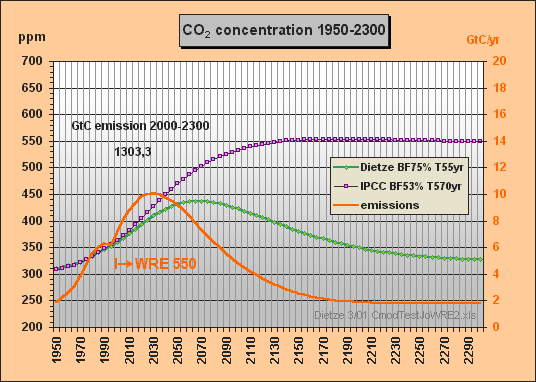
Fig.6: Model results for the WRE550 stabilization scenario till 2300
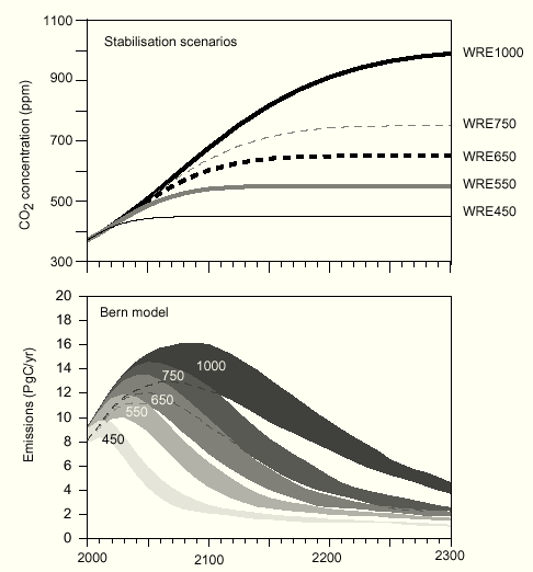
Fig.7: WRE stabilization scenarios computed with the Bern model
Comments:
The stabilization concentration Cs can be easily calculated for given emissions E (GtC/yr) in case the CO2 concentration has reached a constant level and thus the buffer flux turns to zero. The sink flux S then becomes equal to the emissions E. With the buffer factor BF the total excess buffer content B is (Cs280)·2.123/BF. As S is B/T, Cs can be calculated as
As IPCC-related scientists
assert that they used C14 radiocarbon, injected into
the atmosphere by nuclear bomb tests, to "calibrate" the CO2
sink flux, we look at Fig.8
taken from W. Broecker and T-H. Peng [Greenhouse
Puzzles, Part I (1993)] which shows
the fast uptake of a C14 impulse with an
e-fold lifetime of only 16 years. Chemically
C14 behaves similar to the normal C12.
So we can roughly conclude that the Bern model (using a lifetime of 570
years) must be extremely in error.
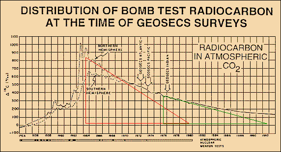
Fig.8: Absorption of bomb-C14 shows an e-fold lifetime of only 16 years
There are two reasons why the CO2 lifetime is not as short as the one of C14. One reason is that C14 slowly decays during its stay in the ocean. So less C14 is gassed out again, and any input vanishes faster. The other (and main) reason is that here indeed we observe a part of the intermixing process with the not so very fast buffer of the upper ocean a process that we cannot observe for normal CO2 emissions, as we are unable to really separate a single impulse. Instead we consider ficticious sections of the total steady CO2 flux which have already passed the distribution phase for the fast buffers. Thus the CO2 excess lifetime is related to the observed sequestration process which we allocate to sink fluxes only and which have to be clearly distinguished from buffering processes. The carbon cycle fluxes in Fig.9 prove that the CO2 excess lifetime is indeed 55 years.
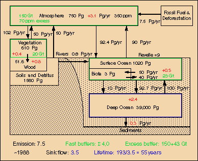
Fig.9: Carbon cycle around 1988 at 350 ppm with 7.5 GtC emissions and 3.5 GtC sink flux
This lifetime should be valid for mid-range, i.e. the 20th and 21st century, the era of fossil fuel use. In Fig.9 the deep oceans (as well as tree trunks and even polar ice which is not included here) are considered as sinks, whereas the other reservoirs (atmosphere, mixed upper ocean layer, soil moisture, light biomass) operate as fast buffers. The excess carbon content of these buffers, i.e. the 20% fraction for a 350-280=70 ppm increment, is specified in green. For the surface ocean the "active" fraction (which takes part in CO2 concentration changes) is reduced according to the Revelle factor. As "light biomass" a fraction of 16% is assumed. The yearly average reservoir additions of carbon are indicated in red. Summed up, the sink flows are 3.5 GtC, which together with the fast excess buffer yield an e-fold time for CO2 of 55 years.
~~~~~
Remarks by Dr. Fortunat Joos: (6 March 2001)
Dear Brian and Tom,
Thank you for your attempts to clarify things to Peter.
Dear Peter,
I believe that the mails by Tom and Brian serve as an answer to your recent e-mails.
Matching within uncertainty of emissions the observed increase in atmospheric CO2 is a minimal test for carbon cycle models. Ocean survey programs such as GEOSECS, WOCE, AJAX, TTO .. produced a huge amount of ocean data: current ocean carbon cycle models are for example tested against the observed oceanic 3-dimensional distributions of
- temperature and salinity (density)
- biogeochemical tracers including phosphate,
nitrate, oxygen, alkalinity, dissolved inorganic carbon, and the carbon
isotope C13
- tracers with a time information including
C14 in dissolved inorganic carbon, CFC-11, CFC-12
and against the observed surface distribution of CO2
partial pressure.
Current carbonate chemistry models employed in carbon cycle models were tested against thousands of water samples analyzed for the relevant quantities such as pCO2, alkalinity, pH, dissolved inorganic carbon, silicate, boron, phosphate ..
Engineering and more real world systems may not be sufficiently described by a single e-folding time scale. An example is the carbon cycle.
With best regards, Fortunat
~~~~~
Remarks by Dr. Brian O'Neill: (5 March 2001)
Dear Mr. Dietze,
I have responded below to what appear to me to be the key points [in your mail] that are leading to your continued misunderstanding of the carbon cycle. While you seem to have a grasp of the mathematical technique of convolution integrals, you are mistaken in your interpretation of how they apply to the carbon cycle, and this is leading you to draw incorrect conclusions on the lifetime of CO2 in the atmosphere. I realize that my response is unlikely to entirely convince you of this. I can only encourage you to more critically assess your own work in light of what the scientific community has learned over the past several decades.
> thank you a lot for
your elaborate response and your very interesting (and revealing) paper
> at Climatic Change
37: 491-503, 1997 MEASURING TIME IN THE GREENHOUSE
> that you sent as pdf,
written together with Michael Oppenheimer and Stuart Gaffin.
>
> To be frank, I was
very upset (and amused) that so little was (and still is) known about the
> carbon cycle, so much
of confusion exists and so many undue and illogic assumptions are
> made.I am baffled
how IPCC pretends to properly having calculated the future CO2
> concentrations. The
idea to consider a big (say 5000 GtC) emission impulse to study the
> nonlinearities from
saturation effects of the ocean chemistry (Revelle factor), is basically
not
> wrong. But you *cannot*
"normalize" the nonlinear response to a small 1 tC, and then solve
> a convolution integral
if many small impulses appear in a time series.
You are correct in your general point that a nonlinear system will respond differently to a large perturbation than a small one. However, this point is not relevant to the specific issue at hand for two reasons. First, most carbon cycle models (including the Bern model) do not use convolution integrals and therefore in no way depend on the results of model responses to a single large emissions impulse. Instead, they solve a set of equations which describe exchange of carbon between reservoirs, as well as other processes such as ocean carbon chemistry and transport processes. Thus they are not subject even in principle to the type of problem you describe.
Second, some models do use convolution integrals (as reasonable approximations of more complete models), but are still valid because the problem you describe does not alter the basic shape of the response of the atmosphere to a single emissions pulse. This shape initial rapid removal followed by slower removal as time passes is not altered by examining smaller and smaller pulses. No matter how small the pulse of carbon added to the atmosphere, ocean uptake still proceeds relatively rapidly at first, when it is dominated by net diffusion into the surface water, and relatively more slowly later on, as ocean carbon chemistry limits net diffusion and uptake proceeds at the slower pace governed by the rate of mixing into the deep ocean. This behavior is fundamental to the carbon cycle and simply cannot be ignored no matter what mathematical approach you take to modeling it.
Should you wish to verify this point, I recommend you construct a simple carbon cycle model (not a convolution integral) that includes carbon chemistry and perform this test yourself. Full model descriptions are available in the scientific literature. You cannot use your own model to do this it will not display this kind of behavior because you ignore carbon chemistry.
> Let me give you a simple example. Cutting
a tree is a very nonlinear function. You cut
> and cut and nothing happens until at last
the tree bends down by 90 degrees. Imagine you
> "normalize" the response. It may be 9 degrees
at the end of every 10% cut. Now I supply
> a "scenario" with five times a 10% cut and
then quit. Your result will be that the tree
> stays bent by 45 degees which is nonsense.
>
> Now imagine we insert a time function with
decay. Suppose, any small cut will heal out
> within two years. So if I make 15 cuts,
each 10%, but within long time intervals > 2yr,
> nothing will happen though according to
the normalized response, the tree should have
> bent by 135 degrees. Believe me as an electrical
and control engineer, that I have
> intensively studied and computed komplex
linear and even nonlinear responses of
> high order systems. This was even an essential
part of my master thesis. You can only
> normalize a response of a linear (or linearized
system within the operating regime). The
> state variables and responses can be composed
from e-functions which are integrated,
> being superposed and time-shifted - by the
so called convolution integral.
> I somehow feel that IPCC still suffers from
prejudices, big misunderstandings, confusation
> and wild imaginations about the carbon cycle.
So it may be not so good for me to read too
> much about their stuff. I am used to think
and analyze by myself. Only in this way you can
> prevent inbreeding and copying IPCC's flawed
parameters. Your conviction that only at
> the 'beginning' of a (small!) impulse the
absorption works with T about 50 yr, but later
> considerably slows down because the mixed
ocean layer becomes saturated, cannot be
> valid. Suppose, after some time the second
impulse arrives while the first one is still
> sequestered. So do you really think, nature
will absorb the last part of the first impulse
> slowly and at the same time absorb the first
part of the 2nd impulse fast ?????? This is
> impossible. Any absorption has to operate
with the same time constant!
Your comments lead me to believe you misunderstand the nature of response functions and the convolution approach you use in your model. The first point of confusion is what the removal timescales we are discussing actually refer to: they describe the adjustment of the CO2 concentration in response to an emission of CO2 from human activity. This is *not* the same thing as the removal of CO2 molecules per se. All [individual] CO2 molecules emitted into the atmosphere are removed in, on average, about 4 years. However, the response of the atmospheric CO2 concentration to emissions from human activity is much slower than that. The reason is that the atmospheric concentration responds to the *net* removal rate (the difference between the carbon flow out of the atmosphere and return flows to the atmosphere) while individual molecules are removed based on the *gross* removal rate (the total flow out of the atmosphere to other reservoirs).
The second point of confusion is how the removal of the effect of a single emission pulse differs from the removal of the overall excess atmospheric CO2. The overall removal can be thought of as resulting from the independent removal of each of a series of individual emissions pulses. Of course this is not how things are happening in the real world the real world is not operating independently on separate portions of the excess CO2 in the atmosphere. The convolution approach simply conceptualizes the overall process this way. Therefore there is no contradiction inherent in a response to a pulse emission that proceeds at different rates over time. Such a function does not imply that after a longer period of continuous emissions, carbon sinks will be removing recent emissions more quickly, and older emissions more slowly, as you conclude. It is simply a means of conceptualizing why overall removal, which applies to all carbon, is occurring at a particular rate.
Some further points that may be helpful in making sense of this: Convolution integrals may seem an odd tool since they are somewhat "artificial" in the sense just described. But it is a useful technique because it can simplify computations and, perhaps more importantly, by deriving the response of the atmosphere to a single pulse in emissions (that is, deriving a "response function") for use in the convolution approach, we can gain insight into how, and why, the carbon cycle responds to emissions under other conditions.
Your argument about the lifetime essentially boils down to a choice between two different response functions. Your own function implies that the effect of a single pulse emission is removed with a constant rate over time, persisting on average for about 50 years. Response functions derived from state of the art carbon cycle models show that the response to a single emissions pulse would be relatively rapid removal at first, followed by slower uptake, with a fraction of the effect of an emission being extremely long-lived and essentially permanent. This overall shape of the response function is a result of basic ocean carbon chemistry, modified to some extent by uptake from the terrestrial biosphere. Without going into detail, removal is initially rapid due to unfettered diffusion into the surface waters, then slows as carbon chemistry increases the concentration of CO2 dissolved in the surface water more than otherwise would be expected, and finally a portion of the effect is essentially permanent because when carbon is added to the atmosphere-ocean system, it causes a shift in the the equilibrium distribution between the two so that when equilibrium is restored, the atmosphere will contain more carbon (relative to the oceans) than it did before.
Of course the response to a single emission pulse cannot be observed in the atmosphere, because the atmosphere has been subject to continuous emissions from human activity for over a century, not to a single emissions pulse. It is therefore impossible to confirm a response function derived from a model either your 50-year response or the more complex response produced by state of the art models by comparison to observations. How then does one decide between the two? One might test the alternative models to see if they can reproduce the observed history of atmospheric CO2 levels. You argue that your own model is validated since it is able to do so. However state of the art response functions can do so as well, so this test is useless in distinguishing between the two.
One might avoid response functions that imply obvious inconsistencies. For example, you argue that it is impossible for pulse emissions of CO2 to be removed at different rates over time, since that would imply that sinks can discriminate between carbon of different ages and remove them at different rates. However, as described above, this argument is based on an incorrect understanding of what response functions actually represent, and therefore is of no help.
Finally, one might choose the response function that is consistent not only with historical atmospheric CO2 data, but also with the greatest amount of knowledge of different carbon cycle processes. An excellent example in this case is carbon chemistry: it is included in state of the art models, but not in yours. It is the primary determinant of the difference in the shape of the response functions if it is included, it implies that uptake slows over time and a portion of the effect of emissions is essentially permanent. Carbon chemistry is very well understood. In order to make a credible argument for ignoring it you need to explain how scientists have somehow gotten carbon chemistry wrong despite countless laboratory experiments and countless measurements in the oceans that support it. You would in fact need to show why fundamental chemical theory that explains many other things besides the distribution of carbon in the ocean is wrong as well. You have made none of these arguments, and your model therefore cannot be considered credible.
Brian O'Neill
~~~~~
Peter Dietze's answer to Dr. O'Neill: (7 March 2001)
Dear Dr. O'Neill,
thank you a lot for your response on 5th March which may essentially help us to come to a compromizing conclusion.
So far we agree re that the response of a *nonlinear* system depends on the size and occurrence time of a CO2 impulse and the past system history and thus cannot be normalized or computed by a convolution integral. But of course, the problem can be solved by a set of analytic equations. Moreover I agree to you, that for a linear (or linearized steady) system the assumption of CO2 impulses is ficticious, as indeed we have a continuous CO2 flux. But it is important to note that because the system is a slow integrator, the flux can be partitioned into emissions impulses and thus we can apply a normalized response function and integrate the time-shifted responses using a convolution integral as I do in my model.
A most important feature that you might not yet have fully realized, is that it makes no difference to process a time-series of impulses, while at the same time we have a basic global CO2 increment left from still unsequestered previous injections in the atmosphere. Everything decays in the same way (with the same time constant) and *independently* superposing each other (i.e. adding of concentration changes). So there is no difference at all whether we take T = excess buffer content / total sink flux or we take the incremental buffer content and the incremental sink flux allocated to any individual impulse (or sum thereof) at any time. This is a basic processing feature of any linear system (or linearized system within the operating regime) - and part of the basic knowledge of control engineers.
You are right that in my model I seem to ignore the ocean carbon chemistry. I seem to ignore as well the cold deep water formation, ocean currents, biological pump, precipitation, the growing and decaying of biomass etc etc. But you are completely wrong in concluding that my model will therefore produce incorrect results. Why? The essential difference between my model and IPCC-affiliated ones is that those try to cope with many known physical and chemical processes and they aim to *compute* the present (and past) global sink flows (which is unnecessary as these are and were observable). They use future emissions scenarios and calculate future sink flows and thus get future CO2 concentrations using the same equations.
Not so my model. As *observed* past global sink flows were used to best-fit estimate the model core parameters, all the real effects are coped for - including the performance of the ocean chemistry during the last century. So the modelled sequestration of my emission impulses, being part of the total global sink flux, is valid "over all" and *comprises* all natural effects that occurred during sequestration of a long sequence of emitted impulses even those effects that are not yet known and that IPCC models are not coping for. This is the reason why my model quite correctly reproduces the (smoothed) measured CO2 curve till to-date and should be expected to do so for the next century as well.
If my model was wrong or based on erroneous assumptions and misunderstandings (putatively caused by not coping with all the body of work of IPCC-affiliated scientists that I was urged to read), it wouldn't perform that well. As long as simplifications are conforming with the physics and chemistry of the bulk uptake processes, a simple model's performance can even outbeat a sophisticated model's where the dynamic properties are unsufficiently coped for.
The clue of my model is that I only consider the *change* in uptake flux which is proportional to the CO2 partial pressure increment against the equilibrium, e.g. 280 ppm. This reflects the acting main physical and chemical laws and thus is valid for the bulk of the sink fluxes, which is well supported by statistical analyses of Dr. Jarl Ahlbeck ( http://www.john-daly.com/ahlbeck/ahlbeck.htm ). All global sink flow observations were best-fit condensed in only two core model parameters (T and BF), which form the "input" to the model, but being by no means assumed or preset.
Actually your point that the Revelle factor acts as to more and more delaying the sequestration of an emissions impulse through the ocean boundary layer and thus a constant "lifetime" cannot be defined, may not really be relevant. We have to cope with a vertical mixing of this boundary layer and a sequence of overlapping impulses. As indeed a permanent CO2 sink flux exists, you could consider my impulses as being fictitiously partitioned in such a way that there is an *effective* lifetime of 55yr which rather keeps constant. I agree that this time constant T would slowly increase, the more we saturate the (partly mixed) ocean, but this is not what you meant - you meant the boundary layer effect. Re the mixed ocean Revell factor, I already stated that with 1,300 GtC in my IS92aD scenario this T-increasing effect will only show up little because of the huge capacity and the thermohaline circulation providing "fresh" water for a long time. Any slight under-linearity in ocean uptake may even be over-compensated by the biomass sink response. The biomass sink is implicitely included in my model.
My conclusion about the vast discrepancies in IPCC's future model responses is that they seem to over-interprete the impact of the boundary Revelle factor and unsufficiently cope with the biological pump and uptake by precipitation, especially with the CO2 sequestration in high latitudes where the cold ocean boundary is very undersaturated. Note that even the outgassing of upwelling water reduces with increasing CO2 concentration.
I am thanking Tom Wigley and Dr. Joos as well for their comments which should mostly been answered herewith.
Best regards,
Peter Dietze
![]()
10 March 2001 (upgraded 31 March), Dipl.-Ing.
Peter Dietze
Phone & Fax: +49/9133-5371
e-mail: p_dietze@t-online.de
this paper: http://www.john-daly/dietze/cmodcalc.htm
![]()
Return to Climate Change Guest Papers Contents Page
Return to "Still Waiting For Greenhouse" Main Page